F:M ratio as a theory is one of the most important aspects in wastewater treatment but also one of the most poorly understood concepts. Occasionally textbook numbers are good guides, however there are many instances in which understanding the complexity of F:M ratio may help to provide further insight. As a consultant it is very common to see strong emphasis on calculations such as F:M ratio. The emphasis on these calculations have the ability to impact potential operational changes we make, however F:M values as shown on paper do not always reflect actual conditions as to how the bacteria behave and may be viewed under the microscope.

F:M Ratio as a Gradient

F:M ratio calculations take the proportion of food (i.e., lbs. of BOD) against the proportion of mass (or microorganism). An overall F:M ratio calculation assumes that the available amount of food is constant throughout the basin. The biggest flaw in this calculation is that all food (i.e., BOD) is not the same. To visualize a true F:M curve one must think of what the actual F:M ratio is at various points in the aeration basin (i.e. very high at the front end and little to no available food on the back end).

All “F” is not the Same

There are many different fractions of BOD including particulate, soluble, and BOD in the form of volatile organic acids. A good analogy for this extends to nutrition and the difference we experience eating “oatmeal” vs drinking “Kool-Aid”. Oatmeal is complex and there are many enzyme reactions that need to occur before it can be taken up in our mitochondria, whereas if you provide Kool-Aid to children at a birthday party, the impacts on their energy levels may often be seen within minutes (as chaos ensues!).

A good visualization technique for this concept is to picture the “mouths” of bacteria (their cell membranes) as a “filter”. Food that is small enough to pass through this filter immediately enters the cell (absorption), while larger “pieces” adhere to the outside of the cell membrane where biochemical reactions occur to process the food to where it can enter the cell. The “smaller the pieces” of food, the higher the actual F:M ratio is in the initial contact zone of the aeration basin.

Septicity/Fermentation Impact on Availability of Substrate

A simple way to look at fermentation reactions versus “complete” treatment of BOD is based upon the availability of an oxygen electron receptor (free or combined). When there is an oxygen source available this is used, Krebs cycle reactions occur, and end productions of new cell mass, carbon dioxide, and ATP (energy) are produced. When there is no oxygen electron receptor available, “full treatment” doesn’t occur, but rather larger “pieces of food” are converted to smaller pieces (think incomplete anaerobic treatment- formation of volatile acids). Substrate such as Acetic acid are immediately available in the aeration basin and generally either oxidized or stored by bacteria within 15-30 minutes of treatment. Therefore, the more septicity that occurs prior to the aeration basin, the more amount of readily available substrate, and the higher amount of readily available “F” there is to meet the RAS in the front of the aeration basin. Note that the BOD concentration itself may not have changed as fermentation occurs, but the food becomes more readily available once it is exposed to septicity.

The “Race” in the Initial Contact Zone

The initial 15-30 minutes of aeration have significant impact in which bacteria gain competitive advantage due to their various kinetic growth rates, storage capabilities, morphology, and other conditions. This small section of the aeration basin is only represented by a sliver in the overall F:M calculation, however it is vital for which bacteria ultimate gain competitive advantages.

Extended Aeration Processes and systems with large Aeration Basins

In systems with high hydraulic retention times, there is often a prolonged period on the “back end” of the aeration basin in which there is low food availability, or often endogenous activity (think “aerobic digestion”/cannibalism). In these systems, it is possible for conditions on the “back end” as well as the front end/ “initial contact zone” to have significant impact on the bacteria which are selected. Dr. Richard described these systems as “dual sludges”. In these systems the F:M ratio often appears low on paper, however it is possible for microbes that gain competitive advantage in the “initial contact zone” to also play a major role in biomass conditions.

BNR and Other Factors 

Due to the complexity of many emerging treatment schematics F:M ratio is further impacted. Examples include reactions in anoxic and anaerobic selectors and well as carbon availability in areas such as post-anoxic zones. In systems such as selectors internal cellular storage may be promoted wherein soluble BOD may be taken up into the cells, however not yet oxidized. Many bacteria also can store substrate in aerobic zones (i.e. PHB granules) in which they can gain competitive advantages over other bacteria when there is a high actual F:M ratio (in terms of high amounts of readily available food).

The” M” Component

The actual amount of available food (“F”) is only part of the equation and many of its complexities are explained above. Factoring in “M” (microorganisms or mass) there are further considerations including inert fractions, fractions of MLSS concentration that are polysaccharide, fractions of MLSS concentration that are protozoan, metazoan etc., and the actual % of bacteria that are alive/viable/ Please note that MLVSS is a better representation of separating inert fractions and does not distinguish between viable and non-viable bacteria). A separate blog at Why the MLSS Concentration is Not Always Representative - Ryan Hennessy Wastewater Microbiology (rhwastewatermicrobiology.com) goes into further detail on understanding how MLSS and MLVSS.

Summary

Overall, process control calculations have their place but are best utilized when combined with accurate microscopy analysis. The bugs do not “lie” and the microscope always helps to tell the full story.

Technical Wastewater Information Resource: https://rhwastewatermicrobiology.com/wastewater-microbiology-book/

In this blog, we are going to deviate from the more technical aspects and more into what I hope are useful tools for career development and success. I have been “around the block” enough that I feel some of these thoughts may be useful to the up-and-coming generation of new wastewater professionals. This article will be written from the perspective of someone completely new to the wastewater industry, however it is likely these thoughts will also be applicable to experienced professionals as well. 

Prior to Applying

I highly recommend job shadowing at a plant prior to applying. This allows a general idea of the culture, what your job responsibilities may be, and if it is something that you want to be a part of. Often if you have a day of job-shadowing, you may be exposed to different people at the facility and you can get a feel for the personalities and the interaction between management and operational staff. Remember that employment is a two-way street and not only are they evaluating you, but you should also be evaluating what you see in them, and whether it would be a good fit. Fortunately, at the time of this writing (October 2023) there is a major shortage of operational staff, and the tables are tilted to be selective in which endeavors you want to pursue.  If you are new to the wastewater field, ideally you want to find a culture that is conducive to training and learning new skills. 

Compatible Skills

It is essential to have a realistic understanding of your personal strengths as well as areas which don’t come as naturally to you. In the wastewater industry, the biggest factor here to consider is mechanical aptitude. The degree to which proficiency in maintenance skills determine success in your job performance is often related to how specified individual work is. For example, in small plants, operators often need a broad range of skill sets, usually including proficiency in maintenance related tasks. You want to make sure you put yourself in the best position for success. Even areas that don’t come naturally for you can eventually become areas of proficiency, however you want to get a feel for the level of support you will have in acquiring these skills. Having people that can serve as mentors significantly reduces the learning curve and improves your chances of success. 

Base Knowledge

Mapping your career trajectory is challenging and if you speak to most wastewater professionals, you will likely find that they entered the wastewater industry by chance rather than as an intended career. Throughout our careers, it is highly likely that our ambitions and goals may change, therefore the broader your knowledge base and skillset, the better the foundation you obtain to align your goals with your circumstances throughout your career. In most instances, this circles back to identifying a proper fit in your first job in which you are exposed to multiple areas and have the necessary support to learn. 

Advice for New Hires

I feel that in the early stages of a new job role building rapport and gathering an understanding of the inter-place work dynamics are crucial. It is generally best to be agreeable, friendly but not an “open book”, and always make sure you are paying close attention to detail and the quality of your work. You want a reputation as someone who works hard and does good work. Expect that anything you say about anyone else will be repeated and find its way back to them. Refrain from topics that may be divisive such as politics and religion and learn about your colleagues’ interests in areas such as sports, recreation, and family activities. Participating in activities outside of work with colleagues is an individual preference, however I personally believe that strengthening these relationships is often not only pleasurable, but also often beneficial for career development. I personally recommend being very guarded about your career aspirations, especially when you don’t know if they put you in direct competition with others.

Other General Guidelines for Workplace Conduct

• Always be in control of your emotions and do not react impulsively.
• Communicate effectively, concisely, and through the proper channels.  
• Gain an understanding of what your authority is to implement decisions, and when to run things by the people you report to. 
• When possible, try things on your own before asking, but also keep the risk to reward aspects in consideration. Generally, management wants to see that you are resourceful and independent, but they also don’t want to have to clean up your mistakes. 
• Maintain good personal hygiene and take pride in keeping your working areas clean and organized. 
• Be truthful, do what you say you are going to do, and be on time. 
• The intimacy of communications should be directly related to the possibility of these communications evoking emotion. For example, if something is straightforward this is generally best through email, while more complex subjects should be talked about in person or over the phone. 
• If you think something you have to say may evoke negative emotion in others, sleep on it. See in the morning if what you had to say is still important enough to bring it up. 

Navigating your Career Path 

There is certainly a balance in the technical aspects as well as the personal aspects of any job. Successful people tend to be proficient in both, as weaknesses in either area will likely limit your opportunities. Once you determine what you want your career trajectory to be, you will want to determine the best path to get there. The beauty is that there is no right or wrong and the right fit for everyone is different. If you have ambitions of advancing you will want to determine if management or technical specialties are your desired area. If your goals are technically oriented, you will want to eventually specialize in these areas and become an expert. If your goals are leadership oriented, you will want to get a feel for the organizational structure of where you work and what that path would look like. In both scenarios, relocation and new employment opportunities are often required. I personally believe that in the early stages of your career you want to put a minimum of 1 year into any employment, don’t ever leave a job without a new job lined up, and do your best to maintain relationships and not burn bridges. It is a small industry, and you will gain a reputation quickly. Lastly, be aware of where your opportunities exist. For wastewater operators there are industrial facilities, municipal facilities, and contract wastewater operation companies as options in which you can work. These can branch off into a wide area of other focuses, and all have their own respective pros and cons. Don’t be afraid to ask for advice, especially from people who have been in the industry for a significant amount of time. Many of us learn the hard way and it is also personally satisfying to help others to not make the same mistakes that we did!

Technical Wastewater Information Resource: https://rhwastewatermicrobiology.com/wastewater-microbiology-book/

Toxicity and Inhibition are two important but distinctly different concepts in biological wastewater treatment processes. While both are viewed as negative, it is important to recognize the differences in these terms. The following will start with an explanation on toxicity and go on to explain the areas of overlap as well as the distinct differences in these terms. 

Toxicity 

Dr. Michael Richard defined toxicity as events in which the oxygen uptake rate (OUR) of the bacteria when fed increasing amounts of a substance, reduced OUR (oxygen uptake rate) values below the “unfed”/ baseline value. For example, if a stable RAS (return activated sludge) sample were collected and DO (dissolved oxygen) depletion over time were measured, this may have an OUR value of around 10 mg/L/hr. When the RAS sample is fed substrate, increases in oxygen uptake rate should increase in correspondence with the amount of added substrate (food). As an example: adding 2 mLs of substrate may result in an increase of OUR from 10 to 15 mg/L/hr., 5 mLs addition may increase the OUR to 25 mg/L/hr., and 10 mLs addition may increase the OUR value to 40 mg/L/hr. representing a “normal/healthy” curve.  In an event in which toxicity occurs, at a certain value of added substrate, the OUR value decreases below the baseline value (in this case 10 mg/L/hr. for an unfed RAS sample). 

In practice, with respirometry testing it is common to see normal correlations of OUR with various amounts of fed substrate until a toxicity “threshold” is reached. There is commonly an initial increase in OUR values due to stress, followed by an often-sharp decline in the OUR value once the concentration of the substance added reaches a toxicity threshold value and bacteria begin to die (dead bacteria don’t use oxygen).

Toxicity may be measured in a wholistic approach (i.e., OUR testing) or may also be more specific to microbes that are impacted by an event (more challenging to test for). It is important to recognize that biological wastewater treatment processes encompass a highly competitive environment for growth, and it is sometimes possible that if a microbe has the capabilities of “filling the void” and competing in an environment that may be toxic to the former microbe, the corresponding impacts on biological treatment performance may be variable. 

Toxic Substances 

Toxicity occurs when the crippling of the given microbe’s enzyme functionality results in death. The most significant factor of any substance is its concentration and impact on the toxicity threshold of the microbial community in the treatment system. Substances recognized as “toxic” tend to have lower concentrations in which they begin to create toxic environments. Most substances are toxic at certain concentrations, however “safer” substances generally are not found in concentrations in which they may have negative impact. Substances most often correlated with toxicity include heavy metals (i.e., chromium, mercury, lead, arsenic), various organic compounds (i.e., solvents, phenols, herbicides, hydrocarbons), petroleum products, pharmaceuticals, chlorinated compounds, and other oxidizers/cleaning agents such as quaternary ammonium compounds and peracetic acid. 

Inhibition versus Toxicity 

Inhibition overlaps with toxicity as it often begins to occur prior to a toxic threshold concentration. Inhibition disrupts the enzyme activity of microbes and delays the rate of treatment. In respirometry testing a curve showing inhibition would show that as a certain amount of substrate is added, the OUR value begins to decrease rather than increase. When the decrease of the OUR value exceeds the initial “unfed/baseline” value of the RAS sample, inhibition technically switches to toxicity when following Dr. Richard’s protocols. Inhibition may have varying degrees of impact on total treatment depending upon how much time is available for the microbes to recover after inhibition occurs.

Most microbes in wastewater treatment processes are responsible for various functions which rely on the ability of their enzymes to work optimally. When inhibition is present, the microbe doesn’t actually die, rather it decreases or in some instances completely stops its functionality until its enzymes are able to perform again. 

Operational Control Strategies

Under most circumstances decreasing the WAS (waste activated sludge) rate allows for a greater “buffer” for stressful events so that even if a certain percentage of bacteria are compromised, enough bacteria may still be functional for maintaining treatment performance. Many plants have success running the MLSS (mixed liquor suspended solids) concentration and the SRT (sludge retention time) values on the higher ends to allow this buffering function. The degree of flexibility for higher SRT and MLSS values generally depends on the hydraulic and solids loading capabilities of the final clarifier (s) as well as the settling characteristics of the mixed liquor (i.e., SVI- sludge volume index). 

Because concentration of a toxin is the most significant parameter, if a known toxic steam is segregated, there are times in which it may bled in slowly at a rate that is safe and under the toxic threshold. Dr. Richard recommended respirometry testing for these decisions, and not to accept any waste that exceeded a 10% reduction in OUR values at any applied rate. In some instances, separation as well as neutralizing the toxin may be achievable (case specific). 

I recommend a microscopic evaluation immediately after the time of an event in question to gauge the overall health of the biomass. Generally, when accessing the overall health and conditions of the bacteria, input from the consultant helps provide direction, while the experience of the operator and their familiarity with the plant is extremely valuable to determine at which degree to implement operational changes. When a notable toxic event has occurred, usually a form of reduced wasting (but still some degree of wasting to rid the system of dead bacteria) yields success provided that the toxic substance doesn’t continue to enter the treatment plant. Dilution (i.e., higher RAS rates or higher flows of known healthy substrate) is also often beneficial. 

Quaternary Ammonium Compounds and “Legacy” Toxicity and Inhibition

While under most circumstances increasing the MLSS and SRT values tends to be successful, a notable exception is when quaternary ammonium compounds(QAC) are present. Quaternary ammonium compounds may have acute as well as chronic (long term) impacts on treatment performance. Chronic inhibition and toxicity often occur when the concentration of QAC compounds bound within the biosolids exceeds 10 mg/. Because of this “legacy” toxicity impact, there are times in which aggressive wasting corresponding with re-seeding of a healthy biomass are warranted so the quats are ultimately removed from the system. Note that aggressive wasting must usually be done in conjunction with re-seeding of adequate bacteria to achieve the growth of desirable bacteria, especially in industrial wastewater treatment processes. 

 As a rule, it is recommended that any treatment plant that receives quaternary ammonium compounds have these compounds neutralized prior to entering biological wastewater treatment. My direct expertise is in microscopy and process control troubleshooting; however I may be contacted directly as I often refer clients to competent professionals that specialize in these areas related to quaternary ammonium compounds.   

Source: https://rhwastewatermicrobiology.com/wastewater-microbiology-book/

I have been to treatment plants that have had settleability issues and seen tables full of settleability tests with various dilutions of MLSS. I believe the intended objective of the diluted settleability test is to see if less biomass would correlate with improved settling; the general idea that if less biomass settles better, then wasting should theoretically improve settleability.

 There is a tremendous factor that is missed in this test, being that factor such as the MLSS concentration, the SRT (sludge retention time), and the F/M (food to microorganism) ratio (particularly in the first 15-30 minutes of aeration, which I refer to as the “initial contact zone”) are all significant components for what drives the selection of the bacteria that grow within the plant. Contrary to popular belief, changes to biomass may occur very rapidly depending upon environmental conditions present. Therefore, if the MLSS concentration is greatly reduced, it is likely that the microbes that compete with the lower MLSS concentration may be greatly different than what were initially present, often worsening problems rather than improving settling.  

Lower MLSS Does Not Always Correlate with Lower SV30 Value

 The idea that “wasting out the sickness (filaments, zoogloea etc.) appears to be prevalent among many wastewater treatment professionals. Our natural intuition is that if the sludge blankets in the final clarifier (s) are high, wasting aggressively would create more room for sludge to settle. Issues such as zoogloea bulking, bulking from low DO filament types, and bulking from various organic acid filament types all have the potential to worsen with increased wasting rates. While these listed issues are separate, the commonality is that selection of undesirable bacteria is based on the bacteria’s high kinetic growth rates and their ability to store food (“hoard it from floc forming bacteria) when there are higher F/M ratios in the initial contact zone of the aeration basin. For example, “low DO” is generally a function of the oxygen availability in proportion to the oxygen uptake rate of the bacteria. A way I like to think about it is that the bugs always want to achieve their desired MLSS concentration based upon the incoming organic loading rate. Therefore, rapidly increasing the wasting rate has the potential to increase bacterial growth rates, increase corresponding oxygen uptake rates, and further increase competitive advantage for Low DO filament types, basically creating a negative feedback loop resulting in higher aeration costs, additional sludge production, risk of loss of nitrification (if desired), and often further weakening the floc structure. 

Importance of Microscopic Evaluation Diagnosis 

Determining the predominant problem of settling issues through microscopic evaluation can be predicted with an extremely high amount of accuracy when it is done by a trained professional. The first (and often easiest step) to is to identify the root cause of the issue. Major problems may arise when the root cause of the problem is mis-diagnosed and the “wrong path” for troubleshooting is chosen. Due to the complexity and overall subjectiveness (sometimes more “art the science”) with wastewater microscopy, it is often cost effective and practical to send a split sample to an expert prior to choosing a troubleshooting strategy. 

Practical Application 

The truth is that there are some problems in which increasing the wasting rate is warranted, and other problems in which decreasing the wasting rate may be warranted. A quick example of when increasing the wasting rate is warranted would be if bulking is caused by filamentous bacteria types that gain a competitive advantage at higher SRT values/ lower food availability on the back end of the aeration basin. 

There is no “one size fits all” approach and each situation must be considered. For these reasons, I do not offer operational suggestions without a discussion with operational personnel about assessing the level of urgency, the treatment plant goals, and other logistics etc. I would personally be highly skeptical of any person or company who is offering advice and/or a product without obtaining intimate knowledge of the individual circumstances of each situation beforehand. 

Furthermore, it is common that more than one change may need to be made at a time for recovery after a treatment plant upset. For example, decreasing the wasting rate when the treatment plant is organically overloaded sounds good in principle, however if the sludge isn’t settling because of filamentous bulking by organic acid filament types, an intervention such as selective RAS chlorination may be needed in conjunction with increasing the MLSS concentration, trying to decrease the incoming organic acid concentrations, changes such as step-feed, etc. 

Source: https://rhwastewatermicrobiology.com/wastewater-microbiology-book/

A brief look at a table demonstrating the various bulking filamentous bacteria types commonly observed in wastewater treatment process will show that a high % of filamentous bacteria (and other bacteria that may potentially be undesirable at certain amounts) are recognized to “proliferate at elevated concentrations of low molecular weight organic acids”. This produces a common question “What are organic acids?”

Organic Acids in Wastewater 

A serviceable analogy for how bacterial cells “eat” is to think of their cell wall as a “filter”. (Dr. Richard liked to describe the cell wall or cell membrane as the “mouth” of the cell). 

In order for “food” to be accessible for the bacteria, it must be in “small enough pieces” that it may pass through the filter. For example, larger “pieces of food” (such as particulate BOD) are not readily available for absorption into the bacterial cell and are retained on the outer edge of the cell (adsorption) while enzymes “break them down” into small enough pieces in which they eventually become available. In wastewater “food” (BOD) is not all the same, and a major component of bacterial selection is how readily available the food is to be utilized by the bacteria.  

Using something like the glycemic index in nutrition as an analogy, Kool-Aid is taken up quickly by cells producing quick and often short-lived energy (ATP), while food like oatmeal is more complex and takes longer to be digested as there are many steps needed to reduce these “larger pieces” into “small enough pieces” in which they may pass through the cell membrane and become available.  

Which Bacteria Compete Best for Organic Acids (Volatile Acids)

Due to the practical analogy of organic acids being “readily available food”, bacteria that have the highest kinetic growth rates as well as the best availability to store food for later (Poly-β-hydroxybutyrate or PHB) gain a competitive advantage when there is a surplus of organic acid/volatile acid substrate (food). Generally, as volatile acid concentrations exceed 80 mg/L, this is where “organic acid” filaments gain a competitive advantage over many floc forming bacteria. Note that previous literature mentions 100 mg/L as a threshold, however we suspect that there are many factors (type or organic acids, temperature, F/M ratio etc.) In addition to certain filamentous bacteria, other bacteria types which may be undesirable at various amounts (i.e., single cell bacteria, zoogloea bacteria types) also favor elevated organic acid concentrations. 

Often, respirometry methods such as oxygen uptake rate may correlate well with a general idea of “how fast the bugs are taking up the food”. A useful and admittedly simple/basic way to think of oxygen uptake rate as it often correlates with organic acids is as “the speed limit”, where at >60 mg/L/hr. undesirable growth may often occur. 

Sources of Organic Acids 

In many industrial wastewater treatment systems and septage, high concentrations of organic acids may be naturally present in the influent. Once organic acids are present, they are “there” and must then be oxidized/treated by bacteria. In areas in which the wastewater become septic and there are no longer available oxygen acceptors (i.e., collection systems, lift stations, holding tanks, primary clarifiers), “fermentation” reactions occur in which “bigger pieces” of food are “broken down”, into “smaller pieces” (organic acids). These fermentation reactions resemble the first stages of anaerobic treatment, however in full/complete anaerobic treatment methane and carbon dioxide are produced as final end products, where formation of organic acids may be generally thought of as “incomplete or partial anaerobic treatment”.  

Organic Acids “Double Edged Sword” 

Having sufficient organic acids is necessary for processes such as denitrification and enhanced biological phosphorous removal, and in some instances treatment plants may even have specific zones (i.e., fermenters) to help convert BOD into organic acids to help produce sufficient readily available food in selector cells. Since septicity and wastewater go hand in hand, there is always a percentage of BOD that is available as organic acids. Lastly, it may be useful to note that in the Krebs cycle, all “food” is eventually converted into acetyl coenzyme A or other intermediates (which requires acetic acid, an organic acid) in which glucose is fully oxidized and energy is stored in ATP and other high energy compounds. (So basically, everything is eventually broken down into acetic acid during “treatment”). Often, where organic acids become problematic, is when they become too highly concentrated in the initial contact zone (first 15-30 minutes) of the aeration basin. There are various short- and long-term operational approaches for troubleshooting problems related to elevated organic acid concentrations and their selection is based on individual circumstances and their logistics. 

Source: https://rhwastewatermicrobiology.com/wastewater-microbiology-book/

There are no general 1 size fits all solutions for troubleshooting biological wastewater treatment system
issues and while it is always preferred to address the root source of a problem, there are simply times in
which this may not be feasible, or logistically practical. A common instance of these scenarios includes
troubleshooting challenges with filamentous bacteria bulking.

Filamentous Bulking Defined

Textbook definition generally defines filamentous bulking as conditions in which the mixed liquor
possesses an SVI (sludge volume index) value of >150 mL/g. This definition often generally applies to
many systems, however the actual SVI values in which clarifier failure is reached (as solids entering the
clarifier at a higher rate than can be removed with corresponding suspended solids carry-over) has many
significant factors such as the size of the clarifier (most specifically the surface area) and the hydraulic
flow rate. For example, there may be treatment plants that are already near or beyond their design
hydraulic capacity and solids loss from the final clarifier (s) may be reached at significantly lesser SVI
values than 150 mL/g in these instances. Vice versa, in situations where the plant is well within range of
its hydraulic capacity and if the clarifier (s) are large enough, higher SVI values may be possible while still
maintaining a low sludge blanket and optimal effluent treatment parameters.

Risk Assessment

It is critical to be able to determine the differences within each system and determine on a scale of 1-10
how severe, or how much risk a potential scenario poses on clarifier performance. In systems such as
municipal systems with high I and I (inflow and infiltration) potential, these large increases of flowrate
must often be taken into consideration in context of how saturated the ground is, and how likely events
such as a heavy rain of a snow melt are to significantly impact the hydraulic flow rate.

RAS Chlorination

RAS chlorination is the process of specifically targeting undesirable filamentous bacteria with
disinfectant (generally sodium hypochlorite) to systematically kill filamentous bacteria to improve SVI
values, while reducing damage to bacteria within the floc as much as possible. In addition to risk
assessment, the choice of RAS chlorination should also be compared to other methods such as sludge
juggling (adding additional basins online etc.), chemical settling aids, and others. RAS chlorination is
generally most successful when flocs are strong and there are high amounts of filamentous extending
from or bridging the flocs together. Microscopic evaluation is important to determine the strength of
the floc structure, the location of the filaments, the overall health of the biomass, and ideally the rank
and abundance of the filamentous bacteria morphotypes that are present in order to assist with
changes in the wasting rate during the period of RAS chlorination.

General Dosing Guidelines

It is important to remember that each system is different, and the chlorine dose required for targeted
kill of filamentous bacteria varies depending upon the chlorine demand brought upon by factors such as
competing reactions. Generally, municipal systems are able to dose much closer to general guidelines,
while various industrial wastewater processes may require significantly higher amounts of chlorine.
Remember to start conservatively with chlorination as the dose can easily be increased, while if the
chlorine is applied to aggressively, this can cause many negative impacts to the health and settling
characteristics of the biomass. It is common for “light” RAS chlorination to involve addition of 2-3 lbs. of
active chlorine per 1000 lbs. MLVSS of the mixed liquor in the aeration basin. Moderate dosages
generally range between 5-6 lbs./1000lbs. MLVSS, and what would be considered generally higher
dosages are >8 lbs./1000lbs. MLVSS.

It is worth mentioning that in rare instances (such as lagoons that are converted to large extended
aeration activated sludge systems) that in these instances we prefer to chlorinate only the estimated lbs.
of MLVSS expected to pass through the clarifier within a 24-hour period. Note that RAS chlorination is
most effective when each “bug” comes into contact with chlorine 1-2x per day minimum. In instances in
which the 1-2x chlorine to “bug” exposure may not be possible options include multiple chlorination
addition points, a hypochlorite “bomb” (which due to high risk is only offered through consulting) or
understanding that a significantly longer period of time may be needed for any potential success (along
with the increased potential that chlorination may not be frequent enough to see beneficial results).
When viewing aerobic biological flocs under fluorescent microscopy, it is common for the majority of
the bacteria within the flocs to be dead or non-viable and the majority of the filaments (often 95% or
greater) to be healthy/viable. In most scenarios, a decrease in the wasting rate is warranted (i.e., 10% or
more) when RAS chlorination is applied due to the fact that filamentous bacteria are extremely efficient at oxidizing/treating carbonaceous organic material (BOD).

Application and Monitoring

It is essential that chlorine is added to the RAS in an area of high mixing. Most often these locations
include areas such as the RAS piping or the center well of the clarifier. The addition of chlorine to locations of poor mixing (such as RAS wet wells) does not allow for even distribution of the chlorine. When calculating the RAS chlorine dose, it is important to adjust the calculations to include the chlorine source (i.e., sodium hypochlorite) to 100% “purity”. The type (s) of filament that is being chlorinated (sheathed versus non-sheathed) have a significant impact in the time needed for improvement in the settleability as empty sheaths with dead filaments often still negatively impact SVI values. When chlorinating the RAS, daily microscopy with phase contrast oil immersion 1000x is desired to monitor the health of filaments. Once 50-60% of filaments show signs such as damaged cells or empty sheaths, the RAS chlorine is generally reduced slightly to prevent over-chlorination.

Additional Notes

Chlorination for filamentous bacteria control is only a “band-aid” option and if the conditions remain in
which filaments outcompete floc forming bacteria, it is common for filaments to grow back rapidly once
chlorination is ceased. Some systems use light RAS chlorine “maintenance doses” to help offset these
challenges, however, this is case specific and depends upon other options available, economic logistics,
availability of operational personnel etc.

Source: https://rhwastewatermicrobiology.com/wastewater-microbiology-book/

There is an interesting and very important correlation with notable differences between the common terms “Low DO” (dissolved oxygen) and septicity. Due to this relatively complex relationship, there is often confusion regarding these terms. The goal of this blog is to briefly explain these differences and how each term should be thought of.

What is Septicity?

In my experience a good way to envision septicity is that “once wastewater has been exposed to septic conditions” it is then forever septic until biological oxidation (treatment). Without going deeply in depth, once available oxygen electron receptors are depleted anaerobic fermentation reactions occur in which carbonaceous “food” is “broken down” into smaller “pieces”, in which we call organic acids or volatile fatty acids. In other terms, once there is no available free dissolved oxygen, or forms of combined oxygen, food (BOD) is converted into simpler and more readily available forms. A good analogy is oatmeal versus Kool-Aid and the differences in how both of these are taken up in your body (Kool-Aid being the organic acids).

Septicity/ Organic Acid Impact on Microbe Competition/ Selection

While the overall loading rate (i.e., lbs./day of BOD) are a factor, the most significant factor appears to be the concentration of organic acids/volatile acids. Literature from Dr. Jenkins and Dr. Richard suggests that bulking from “organic acid filament types” is recognized to occur at volatile acid concentrations >100 mg/L. In addition to filaments, other microbe types that are undesirable at significant abundance (i.e., zoogloea bacteria types, single cell bacteria) appear to have a similar threshold. Based on my personal experience, the 100 mg/L volatile acids concentration appears to be a “ballpark” number due to conditions such as the individual various organic acids that encompass the total volatile acids test. Generally, if organic acid/volatile acid concentrations are diluted below the threshold in which the undesirable microbe gains a competitive advantage, significant changes in the microbes’ present may occur over a long-term period.  Potential control strategies for diluting organic acid concentrations include higher RAS rates, higher internal recycle flows (i.e., BNR plants), implementation of step feed (if possible), and in some instances recirculation of various % of effluent flow to dilute the strength of the incoming wastewater.

Low DO by Definition

The term “Low DO” is relative in that factors such as the oxygen uptake rate and the surplus available oxygen are generally most significant for selection for microbe types we recognize to grow at “Low DO”. A common way to envision this is that when we measure DO, we are measuring “residual DO” that is outside of the floc matrix. The DO setpoint needed to discourage “Low DO” microbe types is based upon the amount of dissolved oxygen needed to maintain aerobic conditions within the interior of the flocs. For example, in lightly loaded municipal systems it is common for DO concentrations as low as 0.5 mg/L to be adequate DO, while in highly loaded systems that are not designed to nitrify the oxygen uptake rate, bacterial growth rates at the front end of the aeration basin are so significant that DO concentrations of 6 mg/L or higher are often needed to discourage Low DO microbes.  For a Low DO microbe type, the applied DO is the most significant factor in controlling the growth of this organism.

Inter-Lap Between Low DO and Septicity

By definition, organic acid microbe types are selected by factors such as the concentration of various organic acids. Applying dissolved oxygen, once organic acids are already formed, is not an effective strategy to oxidize organic acids. Therefore, when troubleshooting a filament or other microbe type that is correlated with organic acids, increasing the DO setpoint is generally not successful if the organic acids are already present in the wastewater being treated prior to the aeration basin.  The only instance in which increasing the available DO is generally successful is if the front end of the aeration basin is septic and organic acids are being formed in the aeration basin itself.

In simple terms, the relationship between low DO and septicity is that once DO is low enough that forms of dissolved oxygen are depleted, fermentation reactions occur, in which organic acids/volatile acids are then produced. In these instances (such as eq basins, collection systems etc.) maintaining aerobic conditions may prevent the formation of fermentation reactions and corresponding formation of organic acids.

Source: https://rhwastewatermicrobiology.com/wastewater-microbiology-book/

It is highly common and often successful to operate activated sludge treatment systems based on maintaining a targeted MLSS (mixed liquor suspended solids) concentration, however as with just about everything in wastewater, there are notable exceptions to the rule. 

What makes up the MLSS?

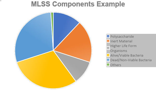
As can be seen from the chart above there are several main components that constitute the mixed liquor suspended solids (MLSS) 

It is important to recognize that MLSS concentration values consist of many variables that may change rapidly depending upon environmental conditions. In our experience the most useful way to envision this is that we are generally attempting to correlate the MLSS concentration to the number of alive/viable bacteria present. Based upon fluorescent microscopy it is common for approximately 40-80% of the mixed liquor to illuminate green (indicating “alive/viable”). 40-80% is a very broad range and depending upon the plant and circumstances that are present these percentages may vary. 

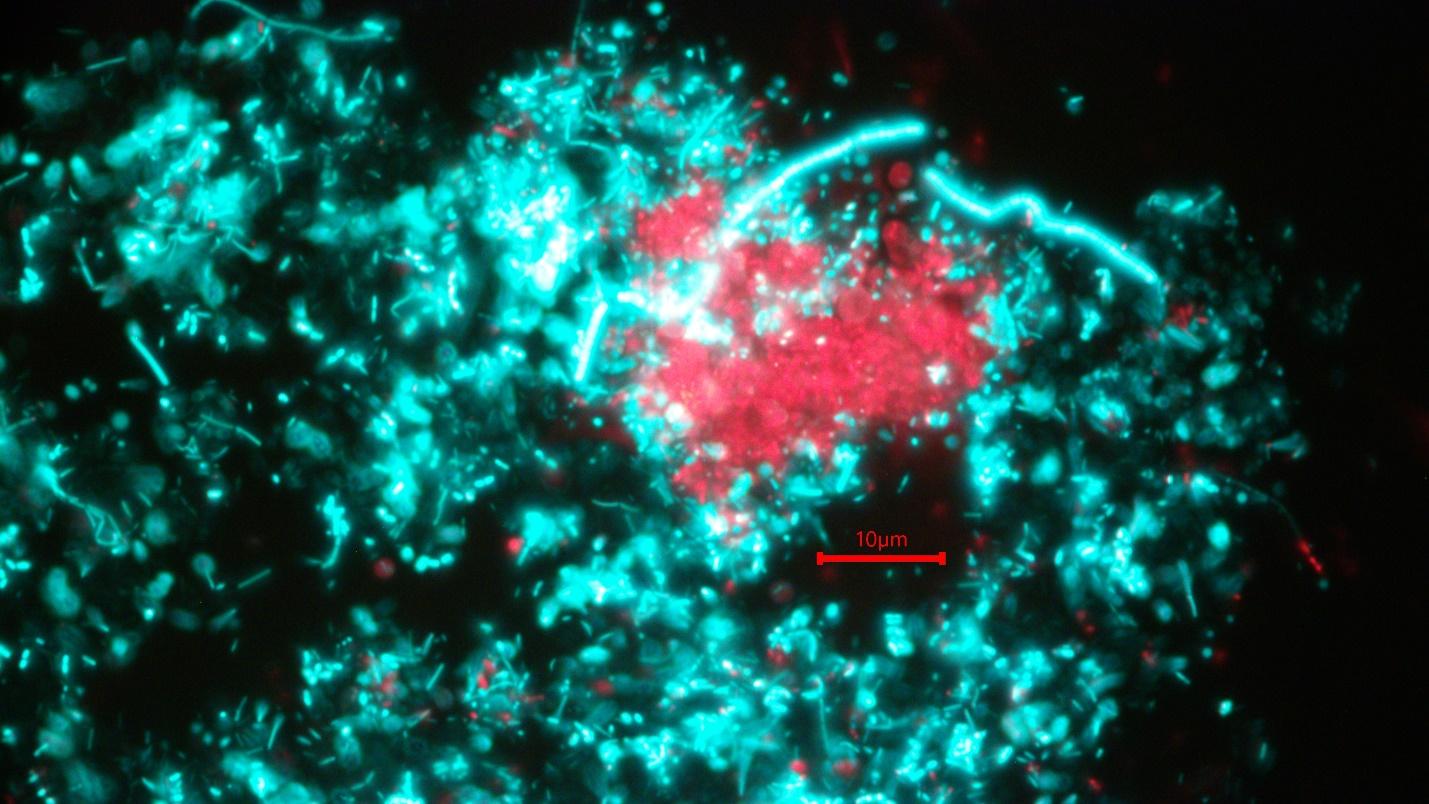
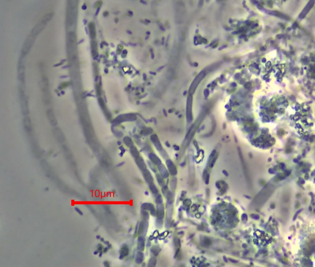
Figure 1: Fluorescent Viability 1000x

The Picture above Demonstrates Alive/Viable (Green) and Dead/Non-Viable (Red)

If we think about the bacterial growth curve ideally in most activated sludge systems, optimal treatment conditions are not optimal growth conditions for the bacteria (specifically that they are on the verge of starvation/endogeny). In our experience it is common for extended aeration systems to have as low as 35-40% bacterial viability, while in highly loaded industrial wastewater processes viability % of 75% or more may be common. Each system is different depending upon the treatment goals, sludge age, temperatures present, and many other conditions. 

Explanation of Other Variables

An influx of inert materials may significantly change the MLVSS (mixed liquor volatile suspended solids) to MLSS ratio. Dead or non-viable bacteria also may possess a biological oxygen demand and if they are now available substrate they may weigh as volatile solids. Higher life form organism weight proportion to the overall MLSS concentration is also recognized to vary between 5-20%. Among other notable variables is temperature and its metabolic impact on the bacteria. In general, at higher temperatures, less bacteria are needed for treatment while when temperatures deplete higher amounts of viable bacteria are commonly needed to achieve treatment goals. 

The Bugs Don’t Lie 

It is always useful to have process control data as part of the “puzzle” to help guide operational changes, however despite what the numbers say on paper, the bacteria present will be representative of actual conditions within the plant should microscopy be performed properly by a trained professional. In summary, when the plant is not behaving as suggested by the MLSS concentration values, it is often due to a change of one of the variables above. Microscopic evaluation, along with in house process control testing, and the input of an operator familiar with the treatment plant and how it generally behaves are most often the best things to get together to help make decisions that are practical and optimize or troubleshoot the system. 

Source: https://rhwastewatermicrobiology.com/wastewater-microbiology-book/

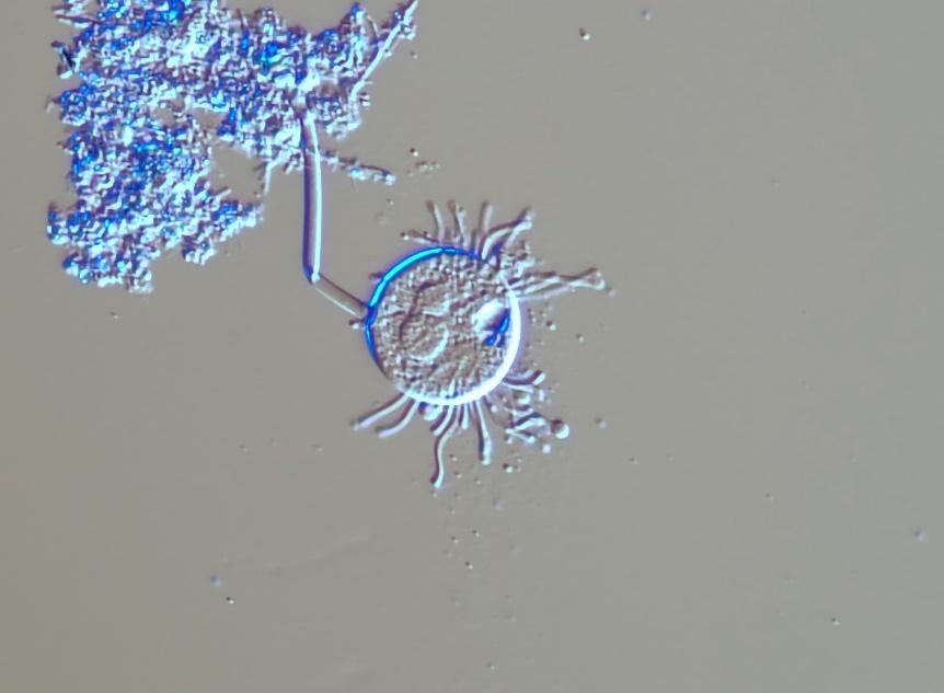
Higher life form organisms such as stalked ciliates and rotifers may be easily viewed under brightfield microscopes. They are fascinating, motile, and easy to recognize however process control changes should not be based strictly upon higher life form organisms and their abundance. The best analogy to use is that “you are what you eat” and if a higher life form organism type is predominant the root cause is that the environmental conditions and the substrate availability favor the selection of this organism. 

Common Examples of why there is NO DIRECT CORRELATION of HIGHER LIFE FORM ORGANISMS ON FM RATIO and SLUDGE AGE

While some general correlations (such as predominance of flagellates often correlating with left over available substrate) often hold true, there are many common situations that may lead operators in the wrong direction. A common example is that rotifers often prey on small floc “fragments”. At higher SRT values when pin floc is present, rotifers are often common, however, if there is a stress that creates de-flocculation it is common for rotifers to proliferate. Nematodes (often associated with high sludge age values) may grow within treatment plants, but also commonly enter treatment processes through the influent, and have been viewed in systems with sludge ages as low as 2 days. There are many other examples that may be viewed at:  https://www.tpomag.com/tags/bug-of-the-month.

How Fast do Higher Life Form Organisms Grow? 

The mix of higher life-form organisms can change quickly depending on their available prey. The longest it takes protozoa to reproduce is 1 day at 20 degrees C (Curds, 1975) so sludge retention time rarely limits their competition. Certain species of rotifers can grow in sludge ages of less than even 4 days (Richard, 2018). In short, there is no proven correlation between higher life form organisms and sludge age, and because there are many other factors besides organic loading that can contribute to changes in sludge condition, basing process control decisions solely on higher life form organisms is not recommended. (Jenkins, 2004)

Impact of Environmental Stresses

From a stress perspective, free swimming and stalked ciliate species are typically the most sensitive to stresses and toxicity while testate amoebae and rotifers can compete well in tougher environments. Note that not all potential stresses are equal and depending on what type of stress is present these can have varying, and sometimes unusual impacts on the microbes present. In most instances, the higher life form organisms are the first to be impacted when there is stress or toxicity. 

Summary 

In summary, there is value in looking at the higher life form organisms but is also important to put their emphasis in perspective as they only represent a “piece of the puzzle”. A shift in predominant higher life form organisms should generally suggest a “deeper look” at what is going on under the microscope with an evaluation that documents factors such as floc structure, dispersed growth, zoogloea bacteria type abundance, filament bacteria type rank, abundance, and suspected growth causes, health of filamentous bacteria, impact of filaments on the floc structure, and bacterial viability within the mixed liquor. 

Source: https://rhwastewatermicrobiology.com/wastewater-microbiology-book/

One of the most challenging problems commonly encountered in biological wastewater treatment processes is sludge bulking due to overabundance of Microthrix filament types.

What is Microthrix?

Microthrix filament types are recognized due to their Gram-positive staining characteristics and are generally 0.8 µm diameter with no visible septa (cell walls). Microthrix are recognized to grow on lipids and long chain fatty acids.  The MIDAS field guide (https://www.midasfieldguide.org/guide/search) recognizes 6 individual species of Microthrix including Microthrix parvicella, Microthrix calidas, and Microthrix subdominas. There are also several closely genetically genera that are strong candidates for Microthrix morphology (characteristics) and similar growth conditions. 

Microthrix Preferred Growth Conditions

• Higher sludge retention time (SRT) values (generally >6 days)
• Oleic acid (formed from septic fats, oils, and grease)
• Colder temperatures 

Common Troubleshooting Strategies

• Reduction of fats, oils, and grease
  • Pretreatment limits on industrial contributors
  • Grease trap ordinances 
  • Primary treatment (i.e., dissolved air floatation) – most common in industrial wastewater treatment plants
• Reducing the SRT value of the mixed liquor
  • Sometimes (but not always) helpful. Note: If there is ammonia limits excessive wasting has the potential to interfere with nitrification
• Selective chlorination
  • Recommended microscopic evaluation first to determine if Microthrix are extending from the flocs
• Settling aids
  • Polymer, coagulants, organic coagulants (jar test first with reputable vendor)

Source: https://rhwastewatermicrobiology.com/wastewater-microbiology-book/